Calculating Weighted Average in Excel.

The concept of average comes from mathematics, average can be defined as the result obtained by adding several quantities together and then dividing this total by the number of quantities.

Usually when we calculate average, we put same weight or priority to each value, this is called un-weighted average.

For example, let’s say we want to calculate the average of Marks of a Student in five subjects:

The marks are as follows:

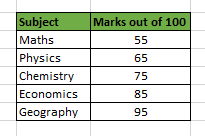
So, we will sum the numbers and divide the result by 5 : (55 + 65 + 75 + 85 + 95)/5 = 75

This is the un-weighted average because in this case we have assigned same significance to each number.

So, what is the Weighted Average then?

Weighted Average is a type of average where item weight is also taken into consideration while finding the average. And because of this one element may contribute more heavily to the final result than another element.

Let’s understand this with the below example:

The marks of the student in 5 subjects are as follows:

Now, let’s consider the student want an admission to an Economics college. So, obviously the college will put more emphasis on the Economics marks and hence they have come up with an idea of assigning weight to each subject as follows.

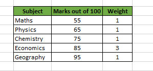
This shows that the college gives 3 times more emphasis on the marks of Economics than another subject, while finding the average.

So, now we find the weighted average of the marks according to the above table as:

((55 x 1)+(65 x 1)+(75 x 1)+(85 x 3)+(95 x 1)) / (1+1+1+3+1)

This comes out to be = 77.85, which is higher than the un-weighted average i.e. 75.

So, in this case the Economics marks have contributed more to the final result than any other element.

How to Calculate Weighted average in Excel?

After understanding the concept of Weighted average in Excel, you must be thinking how to calculate it in Excel.

So, for this you have two methods:

Method 1: Calculating Weighted Average by using Sum Function:

This is an easy method and it requires you to have knowledge of SUM Function. The formula is as follows:

= SUM((1st Element * Weight of 1st Element), (2nd Element * Weight of 2nd Element), … , (nth Element * Weight of nth Element)) / SUM(Weight of 1st Element, Weight of 2nd Element, Weight of nth Element)

Although this method is easier to understand but it is not a feasible option if you have large number of elements.

Method 2: Calculating Weighted Average by using SUMPRODUCT Function [Easy Way]:

This method requires you to have understanding of Excel SUMPRODUCT function. The formula is as follows:

= SUMPRODUCT(, )/ SUM()

An Example on Calculating Weighted Average in Excel:

Below table shows the data from a “Project Task Completion Plan” table.

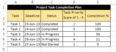
As you can see that, in the above table there are five tasks each one with its own “priority” and “completion percentage”.

So, in this case “Priority” will act as the weight assigned to completion percentage.

Now, to find the weighted Average we can use a formula:

=SUMPRODUCT(E3:E7,D3:D7)/SUM(D3:D7)     [Method 2]

Which results into 61.23

Alternatively, Weighted Average can also be calculated using the formula:

=SUM(E3*D3,E4*D4,E5*D5,E6*D6,E7*D7)/SUM(D3:D7)    [Method 1]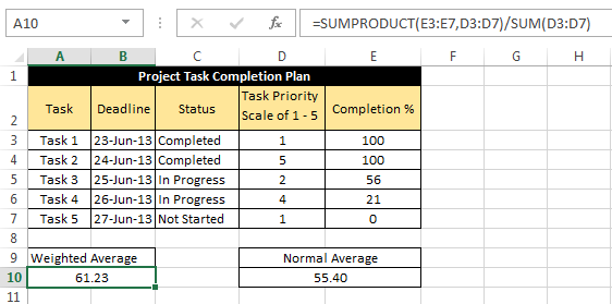

Note: In the above image notice the difference between the result of un-weighted average and weighted average.

So, that was all about finding weighted average in Excel.

Learn more with Excel

Become a Member of Excel Is Fun. :)